 BlackArc
TL;DR
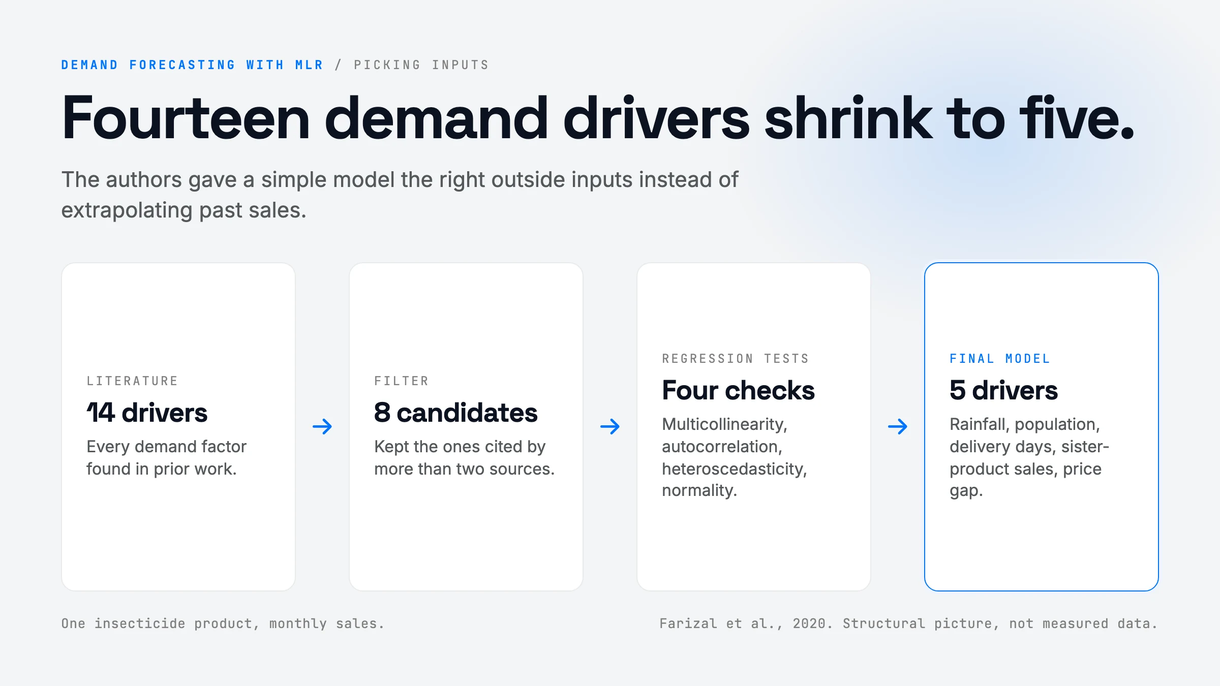
Many consumer-goods companies forecast demand by extrapolating their own sales history, and many of them admit the forecasts are bad. This short conference paper builds a causal forecast instead: a multiple linear regression (MLR) that predicts monthly sales of one insecticide product from outside drivers. The authors start from 14 demand drivers found in the literature, keep 8, and after standard regression diagnostics end with 5: rainfall, population, number of delivery days (their holiday proxy), cannibalization from sister products, and the price difference to competitors. Over 12 months of 2018 the model’s average monthly error (MAPE) is 9.17% against 28.87% for the company’s own forecast. The idea is old and the evidence is thin (one product, one year, no hold-out test reported), but the lesson is useful: before you reach for a fancy model, give a simple model the right inputs.
Problem & Motivation
The pain is concrete. A forecast sits at the top of the supply chain, so a bad number cascades: the factory builds the wrong quantity, distributors hold the wrong stock, and retailers run out or discount. The paper cites a survey of fifty fast-moving consumer goods (FMCG) companies in which most said forecasting did not go as well as they expected, and a common cause was that forecasts ignored promotions, weather, and other outside factors.
The company in this study shows the symptom clearly. Its 2018 forecast for the insecticide barely moves: it stays between about 23,500 and 30,100 units every month, while real sales swing from 13,977 (March) to 38,141 (December). A forecast that hugs a flat line misses every peak and every trough. A pure time-series method (moving average, exponential smoothing, decomposition) can learn a seasonal shape, but it cannot react to this year’s rainfall, a holiday shift that cuts delivery days, or a competitor price cut. Those are causes, and only a causal model can use them.
What’s New (Core Contribution)
Be honest: the method itself is not new. Multiple linear regression for demand forecasting is textbook material. What the paper actually contributes is an applied case:
- A driver shortlist for FMCG demand. Before: practitioners pick inputs ad hoc. Now: a literature screen produces 14 candidate drivers, filtered to the 8 cited by more than two sources (number of consumers, price, cannibalization, income, competitor price, holiday, weather, number of stores). This is a useful starting checklist, though the screen is “count the citations”, not a test.
- A diagnostic-driven reduction from 8 to 5 variables. Before: one big regression with everything in it. Now: the model is pruned using the four classical assumption tests (multicollinearity, autocorrelation, heteroscedasticity, normality), leaving rainfall, population, delivery days, cannibalization, and price difference.
- A head-to-head with the incumbent forecast. The comparison against the company’s real forecast, month by month, is the part worth reading. It shows the size of the gain a simple causal model can deliver over a judgment-based or history-based number.
Not new: the regression, the error metrics, the SPSS workflow. Also not shown: any comparison against a proper time-series baseline (seasonal naive, Holt-Winters, ARIMA), which is the baseline that matters.
How It Works (Technically)
The model is one equation. Everything else is choosing what goes into it and checking that the fit is trustworthy.
Step 1: the general form (equation 5 in the paper).
Y = a0 + a1*X1 + a2*X2 + ... + ap*Xp + error
In plain English: monthly sales equal a baseline (a0) plus a fixed amount for each unit of each driver. Each coefficient ai answers one question: “if this driver goes up by 1 and nothing else changes, how many more (or fewer) units do we sell?” Fitting the model means finding the coefficients that make the squared gaps between predicted and real sales as small as possible over the training months (ordinary least squares). Operationally that is one matrix solve; any library does it in a millisecond.
Step 2: pick candidate drivers. 14 factors from the literature, kept to the 8 that more than two sources mention.
Step 3: run the classical checks and prune. The four tests each guard one assumption that makes the coefficients meaningful:
- Multicollinearity (are two inputs nearly copies of each other?). If number of stores and population rise together, the model cannot tell which one is doing the work, and the coefficients become unstable. Usually checked with the variance inflation factor (VIF).
- Autocorrelation (are this month’s errors linked to last month’s?). If yes, the model is missing a time pattern and its confidence numbers are too optimistic. Usually checked with Durbin-Watson.
- Heteroscedasticity (do the errors grow when sales are large?). If yes, the big months dominate the fit.
- Normality of residuals, which the significance tests assume.
Number of stores, income, and own price drop out here, leaving five drivers.
Step 4: the fitted model. From the paper’s Table 2:
Sales = -277.909 - 12.501*Rainfall + 0.0001*Population + 452.681*DeliveryDays + 0.969*Cannibalization - 3.298*PriceDifference
(The paper’s equation prints -3.289 for the last term; its own coefficient table says -3.298. A typo, but a sign that nobody ran the numbers twice.)
What each term says:
| Driver | Coefficient | p-value | Plain-English reading |
|---|---|---|---|
| Rainfall (X1) | -12.501 | 0.014 | Each extra unit of monthly rainfall costs about 12.5 units of sales. |
| Population (X2) | 0.0001 (rounded) | 0.627 | One extra unit per ~10,000 people. Not statistically significant. |
| Delivery days (X3) | +452.681 | 0.017 | Each extra working delivery day in the month adds about 453 units. This is how holidays enter: a holiday month has fewer delivery days. |
| Cannibalization (X4) | +0.969 | 0.303 | Positive and not significant, which is odd for a variable that should steal sales. |
| Price difference (X5) | -3.298 | 0.000 | The strongest driver (standardized beta -0.652). Each currency unit the product costs above competitors loses about 3.3 units. |
| Intercept | -277.909 | 0.966 | Baseline. Its huge standard error (54,082) says it is pinned down by nothing. |
Two things jump out. First, two of the five kept variables (population, cannibalization) are not significant at the usual 5% level, so the pruning was driven by the assumption tests, not by significance. Second, the price-difference and delivery-days terms carry most of the signal. The authors also report an R-squared of 88.8% for the initial 8-variable model: in plain terms, the inputs together explain about 89% of the month-to-month swings in sales in the fitting data.
Step 5: score it. The paper defines four error metrics. For one month with actual A and forecast F:
- MAPE = average of
|A - F| / A, as a percent. “How far off are we, relative to the size of the month?” The headline metric here. - MSE = average of
(A - F)^2. Punishes big misses hard; units are squared, so hard to read. - RMSE = square root of MSE. Back in units of product.
- MAD = average of
|A - F|. Average miss in units.
Note: in the paper’s monthly tables RMSE and MAD are identical for every row, because for a single month the square root of a squared error is just the absolute error. Only the totals differ.
One trace, end to end (illustrative inputs). The paper does not publish its input data, so take a made-up month: rainfall 250, population 10,000,000, 24 delivery days, cannibalization index 5,000, price difference 1,000.
- Baseline: -278
- Rainfall: -12.5 x 250 = -3,125
- Population: 0.0001 x 10,000,000 = +1,000
- Delivery days: 452.7 x 24 = +10,864
- Cannibalization: 0.969 x 5,000 = +4,845
- Price difference: -3.298 x 1,000 = -3,298
- Forecast: about 10,008 units
Now a holiday month with only 20 delivery days: the forecast drops by 4 x 452.7, about 1,811 units, with no other change. That is the whole value of a causal model: you can see why the number moved and ask “what if”.
Architecture & data flow
flowchart LR
  subgraph Drivers[Monthly driver data]
    R[Rainfall]
    P[Population]
    D[Delivery days / holidays]
    C[Cannibalization]
    PD[Price gap vs competitors]
  end
  H[(Historical monthly sales)] --> FIT[OLS fit]
  Drivers --> FIT
  FIT -->|5 coefficients| M[Forecast equation]
  Drivers -->|next month's values| M
  M --> F[Monthly demand forecast]
  F --> SC[Supply chain plan]
Method pipeline
flowchart TD
  A[Literature scan: 14 demand factors] -->|cited by more than 2 sources| B[8 candidate drivers]
  B --> C[Fit initial MLR, R-squared 88.8%]
  C --> T{Classical assumption tests}
  T -->|multicollinearity, autocorrelation, heteroscedasticity, normality| E[5 surviving drivers]
  E --> G[Final model, Table 2]
  G --> H[Forecast Jan to Dec 2018]
  H --> I[Score with MAPE, MSE, RMSE, MAD]
  I --> J[Compare to company forecast]
The paper's real numbers (Tables 3 and 4). Black: actual 2018 sales. Red: the company's forecast. Blue: the regression forecast. Click a legend item to hide a line; hover a month to see each forecast's percentage error. Notice how flat the company line is.
A what-if calculator built on the paper's fitted equation. Drag the sliders to change each driver; the bars show how much each term adds or removes from the forecast. Input ranges are illustrative because the paper does not publish its input data.
The algorithm, simplified
import numpy as np

DRIVERS = ["rainfall", "population", "delivery_days", "cannibalization", "price_diff"]

def fit_demand_model(history):
    """history: list of dicts, one per month, with each driver plus 'sales'."""
    X = np.array([[1.0] + [m[d] for d in DRIVERS] for m in history])  # [months, 1 + 5]; the 1 is the intercept
    y = np.array([m["sales"] for m in history])                         # [months]
    coef, *_ = np.linalg.lstsq(X, y, rcond=None)   # least squares: minimize sum((y - X @ coef)**2)
    return coef                                     # [a0, a1..a5]

def check_assumptions(X, residuals):
    # The pruning step. Drop or merge drivers until these pass.
    vif = [1 / (1 - r2_of_column_on_others(X, j)) for j in range(1, X.shape[1])]   # >10 = near-duplicate inputs
    dw = np.sum(np.diff(residuals) ** 2) / np.sum(residuals ** 2)                 # ~2 = no month-to-month error pattern
    return {"vif": vif, "durbin_watson": dw}

def forecast(coef, next_month):
    x = np.array([1.0] + [next_month[d] for d in DRIVERS])
    return float(x @ coef)      # baseline + sum of (coefficient * driver)

def mape(actual, predicted):
    actual, predicted = np.array(actual), np.array(predicted)
    return float(np.mean(np.abs(actual - predicted) / actual) * 100)   # the paper's headline metric
The key point is the last line of forecast: the prediction is a sum of named contributions. That sum is what lets a planner explain the number to a sales team.
Built on Prior Work
| Prior idea | What it gave | What this paper changes |
|---|---|---|
| Chopra and Meindl, supply chain stages | Forecasting as the upstream step that drives every later stage | Applies it to one FMCG product line |
| Adebanjo and Mann (2000), FMCG forecasting survey | Evidence that FMCG firms forecast badly, often because they ignore outside drivers | Builds the model that survey implies |
| Chase (2013), demand-driven forecasting | The case for forecasting from demand signals, not shipments | A minimal causal version of that idea |
| Chatterjee and Simonoff, regression handbook | Multiple linear regression and its assumption tests | Uses it unchanged |
| Benkachcha et al. (2013), causal + time-series with neural nets | Combining causal drivers with time-series structure | Drops the neural net; keeps only linear causal terms |
The intro promises “a combination of time series and causal techniques”. In the reported model there is no time-series component (no lag, no trend, no seasonal term). The time dimension enters only through drivers that happen to be seasonal, like rainfall and delivery days.
Results & Evidence
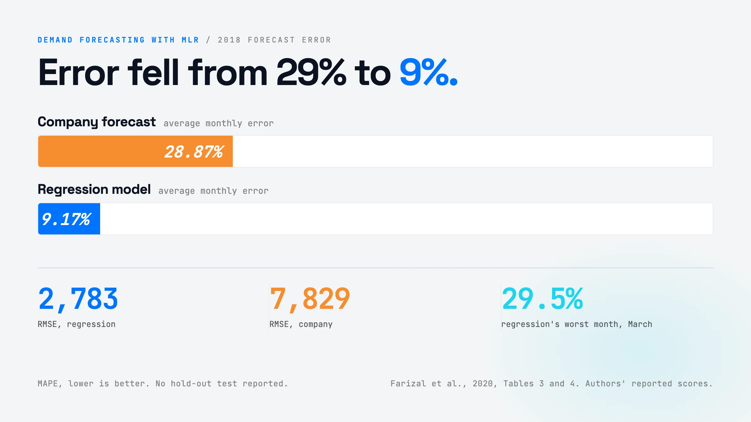
Headline: across January to December 2018, the regression’s average monthly MAPE is 9.17%; the company’s is 28.87%. That is roughly a 3x reduction in error.
| Metric (12-month total) | Regression model | Company forecast |
|---|---|---|
| MAPE | 9.17% | 28.87% |
| MSE | 7,745,689 | 61,292,586 |
| RMSE | 2,783 | 7,829 |
| MAD | 2,246 | 7,468 |
Two more things the tables show, computed from the paper’s own monthly figures:
- Annual volume. Actual 2018 sales total about 344,000 units. The regression totals about 342,900 (0.3% low). The company totals about 313,500 (about 9% low). So the company under-forecast the year by roughly 30,000 units on top of missing the shape.
- Where the model still misses. March (29.5% off) and July (20.7% off) are the regression’s worst months. March is the lowest-sales month, so a small unit error becomes a large percentage.
What the evidence does not establish:
- No hold-out test is reported. The paper does not say which months the model was fitted on. If 2018 was part of the fitting data, the 9.17% is an in-sample number and overstates real forecasting skill. This is the biggest open question.
- One product, one company, one year. Twelve data points of evaluation is a small sample.
- Weak baseline. The only comparison is against the company’s own forecast, which looks close to flat. There is no seasonal-naive, exponential smoothing, or ARIMA baseline. A seasonal method might close much of the gap with no driver data at all.
- Inputs are treated as known. To forecast next month you need next month’s rainfall and competitor prices. The evaluation appears to use actual values, which flatters the model. In live use you would feed forecasts of those drivers, and their errors would add to yours.
- Fragile coefficients. Two kept variables are not significant, the intercept is undetermined, and the cannibalization sign is the opposite of intuition. The model may be fitting noise in a small sample.
- Missing details. The paper never states the units of rainfall, cannibalization, or price difference, or the size of the training set.
Fair read: a believable, directionally right case study, not proof that MLR beats good time-series methods.
How You’d Use It
The transferable lesson is not “use linear regression”. It is: a simple, explainable model with the right outside drivers often beats both gut-feel numbers and fancier models fed only their own history. Here is where that fits.
Your automations and business processes. If you run any repeating plan (inventory reorders, staffing for a support queue, cloud capacity, ad spend pacing), you probably forecast it from last period plus a fudge factor. Slot in a small regression step in the planning pipeline: pull the drivers you already have (calendar working days, holidays, price changes, a weather API, marketing calendar), fit weekly, and publish the forecast with a per-driver breakdown. Cost: a day or two to assemble the driver table, then minutes per run. It pays off when you have at least two or three dozen periods of history and drivers that genuinely change period to period.
Your applications. If you ship a product that helps users plan (a shop dashboard, a booking tool, a budgeting app), “explainable forecast” is a feature people trust. A linear model can say “sales will drop about 1,800 units next month because there are four fewer delivery days”. A gradient-boosted model or an LLM cannot say that as cleanly. Use the what-if form shown above as the UI: let users drag a price or a promo and watch the forecast move.
Your harness. Agents that do planning or ops work often guess numbers. Give the agent a forecasting tool instead: a function that fits or loads a small regression and returns the forecast plus each driver’s contribution. The agent’s job becomes collecting driver values and explaining the result, which is what LLMs are good at, while the arithmetic stays deterministic and auditable. Add a guardrail that rejects forecasts when inputs fall outside the range seen in training.
Your workflows and methodologies. Use this as a baseline discipline. Before you build an ML or LLM forecasting system, fit the dumbest causal model first and score it with MAPE on held-out months. If the fancy model cannot beat it by a clear margin, ship the simple one. The paper’s real lesson is that the company’s process was the weak point, not the lack of a sophisticated algorithm.
Build Your Own (Minimal Recipe)
Smallest useful version, about a day of work:
- Assemble a monthly (or weekly) table. One row per period: sales, plus 3 to 8 candidate drivers. Start with the free ones: working days and holidays (any holiday calendar library), your own price and any competitor price you track, promotions on or off, and weather if the product is weather-sensitive (Open-Meteo has free historical data).
- Split by time. Fit on everything except the last 6 to 12 periods. Never shuffle time-series rows.
- Fit OLS with
statsmodels.OLS(it prints coefficients, p-values, R-squared, and Durbin-Watson in one summary).scikit-learn’sLinearRegressionworks if you only need predictions. - Check the assumptions.
statsmodels.stats.outliers_influence.variance_inflation_factorfor collinearity; the Durbin-Watson value in the summary for autocorrelation; a residual-vs-fitted plot for heteroscedasticity. - Add one time term. Month-of-year dummies or last period’s sales as a feature. This is the “time series plus causal” combination the paper promises but does not deliver.
- Score on the held-out periods with MAPE and MAD, against two baselines: last year’s same period (seasonal naive) and your current process.
- Ship the decomposition. Output the forecast plus
coef * valueper driver, so people can see why.
The two genuinely hard parts:
- Getting future driver values. Delivery days and planned prices are known ahead; weather and competitor prices are not. Use forecasts or scenarios for those, and measure the error that adds.
- Too few rows for too many drivers. With 24 to 36 months of data, five drivers is already a lot. Keep it small, or use ridge regression (
sklearn.linear_model.Ridge) to stop coefficients from swinging wildly.
How to Improve It
- Run a real hold-out test. Fit on 2015 to 2017, forecast 2018 month by month with a rolling origin. Report out-of-sample MAPE. This alone would tell you whether the 9.17% is real.
- Add the missing baselines. Seasonal naive, Holt-Winters, and ARIMA with the same drivers as external regressors (ARIMAX or
statsmodelsSARIMAX). If the causal terms still add skill on top of a seasonal model, that is a much stronger claim. - Combine time and cause properly. Use a regression with ARIMA errors, or a model like Prophet with regressors, so seasonality and trend are learned explicitly and the drivers explain the rest.
- Pool across products. One product gives 12 to 36 rows. Fit a hierarchical (mixed-effects) or global gradient-boosting model across many SKUs, so shared drivers like rainfall and holidays are learned from far more data. This is where LightGBM-style global models usually win in retail forecasting competitions.
- Forecast ranges, not points. Report an 80% prediction interval from the regression. Inventory decisions depend on how uncertain the number is, not just the number. Then test the business value directly: simulate stockouts and holding cost under each forecast, which is a better score than MAPE.
Glossary
- FMCG (fast-moving consumer goods) — cheap, frequently bought products such as soap, snacks, and insecticide.
- Causal forecasting — predicting from drivers that cause demand (price, weather, holidays) instead of from past sales alone.
- Time-series forecasting — predicting a value from its own history (trend, seasonality, recent levels).
- Multiple linear regression (MLR) — a model that predicts one number as a baseline plus a weighted sum of several inputs.
- Coefficient — the weight on one input: how much the output changes when that input rises by 1.
- Standardized beta — a coefficient rescaled so inputs with different units can be compared for strength.
- Ordinary least squares (OLS) — the standard way to fit a regression: pick weights that minimize the sum of squared errors.
- R-squared — the share of the variation in the output that the model explains (0 to 1).
- p-value — roughly, how likely a coefficient this large would appear by chance if the driver had no real effect; below 0.05 is the usual bar.
- Multicollinearity — two or more inputs that move together, which makes their separate coefficients unreliable.
- VIF (variance inflation factor) — a number per input that flags multicollinearity; above about 5 to 10 is a warning.
- Autocorrelation — errors that are linked from one period to the next, a sign of missing time structure.
- Durbin-Watson statistic — a test for autocorrelation; near 2 means none.
- Heteroscedasticity — error size that changes with the level of the output.
- Cannibalization — sales one of your products takes from another of your own products.
- MAPE — mean absolute percentage error: the average miss as a percent of actual.
- MSE / RMSE — mean squared error and its square root; punish big misses more than small ones.
- MAD — mean absolute deviation: the average miss in units.
- In-sample vs out-of-sample — scoring on data the model was fitted on versus data it never saw. Only out-of-sample tells you forecasting skill.
- Seasonal naive — the baseline forecast “same as the same month last year”.
- SPSS — IBM’s point-and-click statistics package, used here to run the regression.