 BlackArc
TL;DR
Linear attention models (Mamba, DeltaNet, xLSTM and friends) squeeze the whole context into one fixed-size matrix, so they are cheap at long context. The catch is how that matrix gets revised. Plain additive writes grow without bound; the popular delta rule fixes growth but, when it rewrites the value at one key, it also disturbs every other value whose key overlaps. The Kronecker Delta Rule corrects only the scalar association between the current key and value, and moves the memory only along the rank-one direction v kᵀ. Other memories change only if they overlap with the new pair in both key and value. Wrapped into a gated block called KronLSTM, it gives the best average accuracy among five strong linear-attention baselines at 1.5B parameters / 100B tokens (59.7 vs 58.1 Avg-6 for the next best), the best real-world recall average, and its lead on needle-in-a-haystack retrieval grows as context gets longer. One clear weak spot: a synthetic repeated-noise needle task (S-NIAH-1) where it does much worse than DeltaNet.
Problem & Motivation
Softmax attention keeps a key-value cache that grows with every token, so long-context inference gets expensive in both memory and compute. Linear attention replaces that cache with a fixed d_v × d_k matrix S that is updated once per token and read with a query. Constant memory, linear time.
The hard part is how you write into S:
- Hebbian / additive writes (
S += v kᵀ, used by mLSTM, Mamba, RWKV under a forget gate) only add. Nothing old gets revised, it just gets buried, and the matrix grows with sequence length. The usual fix is a forget gate, but to remember the start of a long document that gate has to sit near 1, which means little forgetting and more growth. xLSTM’s mLSTM adds normalizer and stabilizer states to keep things in range, and those ratios of large numbers themselves blow up under stress (the paper’s Figure 2 shows mLSTM gradient-norm spikes at high learning rate while KronLSTM stays flat). - Delta-rule writes (DeltaNet, Gated DeltaNet, Kimi Delta Attention) first read what is stored at key
k, then overwrite it towardv. That bounds the memory and gives stable training. But the correction is the whole residual vector(S k − v), written along keyk. Every stored item whose key overlaps withkgets that residual added to it too. In a long context with thousands of items crammed into a 128×128 matrix, keys overlap a lot, so each write quietly corrupts older facts.
The pain in one sentence: fixed-size memories have to choose between unbounded growth and collateral damage on every write, and both get worse the longer the context.
What’s New (Core Contribution)
- The Kronecker Delta Rule (new update rule). Before: the delta rule makes
S kequalv, correcting a wholed_v-dimensional vector. Now: the rule makes the scalarvᵀ S kequal a targetc(usually near 1), correcting one number along the directionv kᵀ. Genuinely new as a memory write in this family; mathematically it is the old Widrow-Hoff delta rule applied to the flattened memory with the Kronecker productk ⊗ vas the input, which is where the name comes from. - Interference that needs a double overlap. Before: delta-rule damage to an old item scales with key overlap alone. Now: damage scales with key overlap times value overlap, so an old item is safe if either its key or its value is orthogonal to the new pair. They also prove that, at the “Newton” step size, this is the smallest possible correction in Frobenius norm and the only one that touches only the addressed key and value directions.
- KronLSTM (architecture). The rule wrapped like other modern mixers: per-key-channel forget gate, a sigmoid erase gate
β, a separate sigmoid write gatec, output gate, short convs, L2-normalized q/k/v, RMSNorm. No normalizer or stabilizer state is needed (unlike mLSTM). The erase and write are decoupled soβsets how much to erase andcsets how much to write. - Stability proofs. Under a long i.i.d. stream, the memory is a Markov chain with a unique steady state whose mean is the least-squares memory, and the expected memory norm is bounded by a data-dependent constant at every step, not just in the limit. Useful, but it is the expected-value story under i.i.d. inputs; real text is not i.i.d.
Repackaged rather than new: the gating recipe (forget-gate parameterization from Mamba / Gated DeltaNet-2, decoupled erase/write like GDN-2), and the chunkwise-parallel training trick, which carries over from DeltaNet unchanged because the transition matrix keeps the same Householder form.
How It Works (Technically)

The memory and the read. Each head holds a matrix S of shape d_v × d_k (128×128 here). Reading with query q returns h = S q, a value vector. You can think of S as a sum of outer products v kᵀ: each one says “when you see something like key k, return something like value v.”
Three ways to write the pair (k, v):
- Hebbian:
S ← S + v kᵀ. Just add. Never revises. - Delta rule:
S ← S − β (S k − v) kᵀ. Read what keykcurrently returns (S k), subtract the error vector from it. This is one step of gradient descent on½‖S k − v‖². The update direction depends on what is already in memory (S k), so it carries old content into other places. - Kronecker Delta Rule (equation 3):
S ← S − β (vᵀ S k − c) v kᵀ.
Plain English for (3): vᵀ S k is one number, “how strongly does the memory currently link k to v?” Call the gap from the target r = vᵀ S k − c. The update adds −β r copies of v kᵀ. If the link is too weak, add some v kᵀ; if too strong, remove some. The direction of the change is built from the input pair alone, never from the memory’s current content. That is the whole trick.
Split it the way the paper does: S ← S − β (vᵀ S k) v kᵀ + β c v kᵀ. The first term erases whatever strength the pair already had; the second writes fresh strength c. With c = 1 you store at unit strength; with c = 0 you delete the association.
Why “Kronecker”. Flatten the matrix into a long vector s = vec(S) and define a = k ⊗ v (the Kronecker product, which is just vec(v kᵀ)). Then vᵀ S k = aᵀ s, and equation (3) becomes s ← (I − β a aᵀ) s + β c a. That is exactly the 1960 Widrow-Hoff least-mean-squares rule with input a and scalar target c. Because the transition (I − β a aᵀ) has the same generalized-Householder shape DeltaNet uses, DeltaNet’s chunkwise-parallel GPU training applies with a in place of k.
Error correction. Show the same pair again and the gap shrinks by a factor (1 − β ‖a‖²). With L2-normalized keys and values, ‖a‖² = ‖k‖²‖v‖² = 1, so the gap shrinks by (1 − β). With β = 1 (the “Newton step”) the association hits the target in one write. With β ∈ (1, 2) the transition gets a negative eigenvalue, which is the known trick that lets delta-rule models do state tracking (parity, permutations); KronLSTM uses β = 2σ(·) for those tasks.
Interference (equation 5), the core claim. For any older pair (kᵢ, vᵢ), the write changes its association by
Δ(vᵢᵀ S kᵢ) = −β r · (vᵢ · v) · (k · kᵢ)
Plain English: the damage is the product of how similar the values are and how similar the keys are. If either is near zero, the old fact is untouched. For the delta rule, the read-out S kᵢ of any old key moves by −β (S k − v)(k · kᵢ): key overlap alone decides, and the moved vector is the whole residual, which itself contains leftovers of other memories. With random 128-dim unit vectors, overlaps are around 0.09, so a product of two is roughly ten times smaller than one.
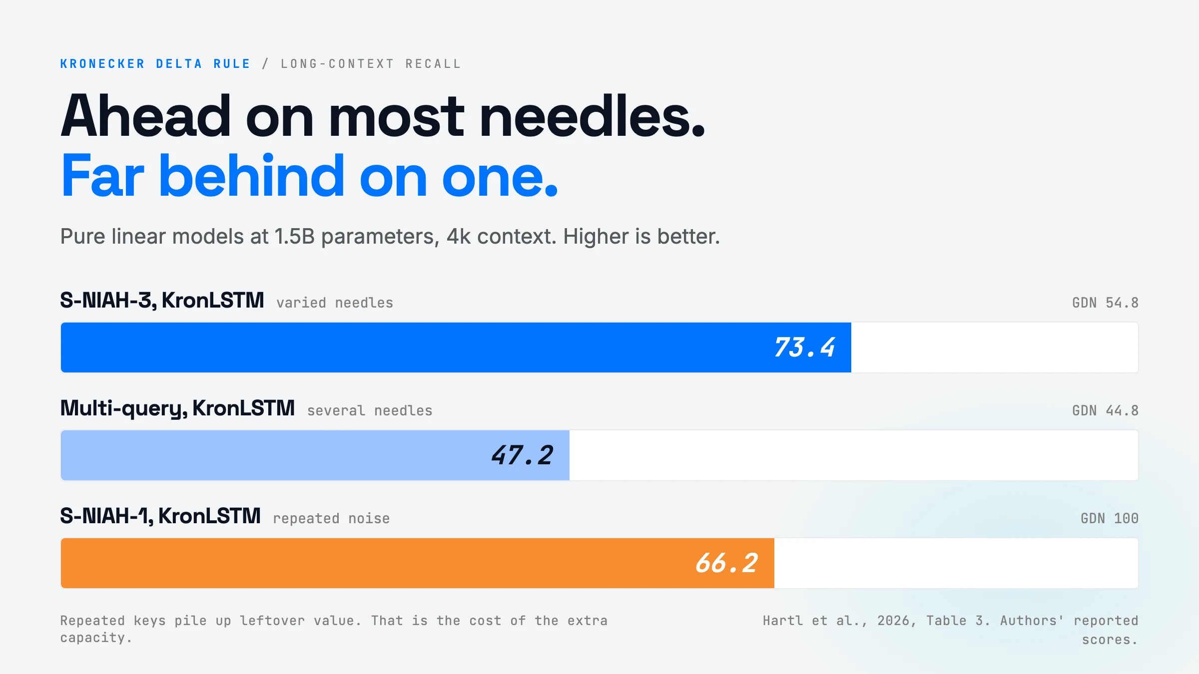
Capacity. The delta rule stores at most d_k exact key-to-vector maps. The Kronecker rule stores up to d_k × d_v exact scalar associations, one linear constraint each. A side effect: one key can hold several orthogonal values, and reading S k returns their sum. This cuts both ways. It is extra capacity, but it also means writing a new value at a repeated key does not wipe the old value’s orthogonal part. The paper blames exactly this “residual accumulation for recurring keys” for its bad S-NIAH-1 score.
Stability (Theorems 1 and 2), in plain terms. Treat a long context as a stream of random (k, v, c) triples. Then:
- The average memory moves geometrically toward the least-squares memory
S_LS, the single matrix that best fits allvᵀ S k ≈ cconstraints at once. So the rule is unbiased: on average it ends up at the best fixed memory for the data. - The memory itself never settles to a point (each new token jiggles it), but its probability distribution converges to a unique steady state whose mean is
S_LS. - If each update is non-expansive (
β ‖a‖² ≤ 1, guaranteed in KronLSTM by normalization and a sigmoidβ), the expected squared memory size is at most4 E[c²] / λ_minfrom the first token and decays toE[c²] / λ_min.λ_minis the smallest eigenvalue of the averagea aᵀ: roughly how evenly the inputs cover the memory’s directions. Translation: memory size is capped by a constant that depends on the data, not on how long the sequence is. No normalizer state needed. - The appendix also shows the slowest-decaying memory mode lasts about
dtimes longer than DeltaNet’s for isotropic normalized values: things stick around longer.
The KronLSTM layer (equation 10). Per head, per token:
S ← S F − β (vᵀ S F k) v kᵀ + c v kᵀ
F = diag(f): a per-key-channel forget gate,f = (1 − σ(W_f x))^awith a learned per-head exponenta, so heads can live at very different timescales.β = σ(w_β · x): scalar erase gate in (0, 1).c = σ(w_c · x): scalar write gate in (0, 1). Usingcdirectly instead ofβ cdecouples erase from write.- q, k, v come from linear layers, a short causal depthwise conv, SiLU, then L2 normalization. Read
h = S q, multiply by a sigmoid output gate, per-head RMSNorm, then the output projection.
It is a drop-in replacement for the attention sublayer of a Transformer block.
Architecture & data flow
flowchart LR
  X[Token input x_t] --> P[Linear + short conv + SiLU]
  P --> N[L2 normalize q, k, v]
  X --> G[Gate projections]
  G -->|f per key channel| M
  G -->|beta erase, c write| M
  N -->|k, v| M[Kronecker Delta Rule update of S]
  N -->|q| R[Read h = S q]
  M -->|memory S_t| R
  G -->|o output gate| O[Gate + RMSNorm + out proj]
  R --> O
  O --> H[Layer output h_t]
flowchart TD
  S0[Memory S] --> F1[Decay: S times diag f]
  F1 --> A[Measure link: v^T S k, one number]
  A --> E[Erase: subtract beta times link along v k^T]
  E --> W[Write: add c along v k^T]
  W --> S1[New memory S]
  S1 -->|next token| F1
  S1 --> Q[Query read S q]
Live toy simulation (not the paper's data). A small memory holds N random unit-vector pairs. One new pair is written. Bars show how much each older pair's stored association moves under the delta rule (red) and the Kronecker Delta Rule (blue), applied to the same memory. Click to resample; drag the slider to change dimension.
Live toy simulation: memory size over a long stream of random unit-norm pairs. Pure Hebbian writes grow without bound; the delta rule and the Kronecker Delta Rule both settle to a bounded steady state, as Theorem 2 predicts for the Kronecker rule.
The algorithm, simplified
import numpy as np

def l2(x):
    return x / (np.linalg.norm(x) + 1e-6)

def kronlstm_step(S, x, W):
    """One recurrent KronLSTM step for one head.
    S: [d_v, d_k] memory.  x: [d] token input.  W: dict of weight matrices."""
    q = l2(silu(W["q"] @ x))                 # [d_k]  (short conv omitted)
    k = l2(silu(W["k"] @ x))                 # [d_k]
    v = l2(silu(W["v"] @ x))                 # [d_v]

    f = (1 - sigmoid(W["f"] @ x)) ** W["a"]  # [d_k] forget per key channel, a > 0
    beta = sigmoid(W["beta"] @ x)            # scalar erase strength in (0,1)
    c = sigmoid(W["c"] @ x)                  # scalar write strength in (0,1)
    o = sigmoid(W["o"] @ x)                  # [d_v] output gate

    S = S * f[None, :]                       # forget: decay each key direction
    link = v @ S @ k                         # ONE number: how strongly k -> v now
    direction = np.outer(v, k)               # rank-one, built from input only
    S = S - beta * link * direction          # erase the old strength of this pair
    S = S + c * direction                    # write the new strength

    h = S @ q                                # read: [d_v]
    return S, rms_norm(o * h)

# Contrast: the delta rule moves S along (S @ k - v), a full vector that
# depends on what is already stored, so it smears into overlapping keys:
#   S = S - beta * np.outer(S @ k - v, k)
Training uses a chunkwise-parallel version of this loop (same math, matrix-multiply friendly), adapted from DeltaNet with a = k ⊗ v playing the role of the key.
Built on Prior Work
| Prior idea | What it gave | What this paper changes |
|---|---|---|
| Fast weight programmers (Schmidhuber 1992), linear attention (Katharopoulos 2020) | Context compressed into an outer-product matrix memory | Same memory, new write rule |
| Widrow-Hoff delta rule (1960) | Error-correcting LMS update | Applied to the flattened memory with input k ⊗ v and a scalar target |
| DeltaNet / Gated DeltaNet / KDA (Schlag 2021, Yang 2024-25, Kimi 2025) | Bounded memory by overwriting S k toward v; chunkwise-parallel training | Corrects a scalar instead of a vector; interference needs key AND value overlap |
| Gated DeltaNet-2 (2026) | Separate erase and write gates, power-sigmoid forget gate | Reused; the difference is the update direction |
| xLSTM / mLSTM (Beck 2024) | Exponential gating, matrix memory, the family KronLSTM joins | Drops the normalizer and stabilizer states; stability comes from the rule itself |
| State-tracking via negative eigenvalues (Grazzi 2025) | β ∈ (0, 2) lets delta models track parity / permutations | Carried over unchanged |
Results & Evidence
Setup: 1.5B-parameter models, 24 layers, 16 heads, d_k = d_v = 128 for all, trained on 100B tokens of FineWeb-Edu at 8k context, same data, tokenizer, optimizer, and seed for every model. Only the mixer differs. Each architecture is tested pure-linear and as a hybrid with sliding-window attention (5 linear : 1 SWA, window 2048).
- Language modeling (Table 1). Linear: KronLSTM Avg-6 59.72 vs KDA 58.12, GDN-2 57.94, GDN 57.73; LAMBADA perplexity 11.72 vs 12.54 best rival. Biggest gains on HellaSwag (+1.7), ARC-e (+2.2), WinoGrande (+2.6). Hybrid: 59.56 vs 58.79 (GDN-2).
- Real-world recall at 2k (Table 2). Linear average 30.31 vs 29.81 (GDN), hybrid 37.40 vs 36.96 (Mamba-3). Small but consistent; it does not win every task (loses TQA, NQ, DROP in the linear setting).
- Needle-in-a-haystack, RULER (Table 3). Linear models at 4k: S-NIAH-3 73.4 vs 54.8 (GDN), MQ 47.2 vs 44.8. Gaps shrink at 16k where everyone collapses (S2: 16.0 vs GDN 17.8). The big exception is S-NIAH-1: KronLSTM 66.2 / 29.4 / 11.6 at 4k/8k/16k against GDN 100 / 100 / 99.2. Linear KronLSTM is worst of all six models here. The authors call S1 artificial (repeated noise sentences) and blame residual build-up on repeated keys. In the hybrid setting the story flips: every baseline’s S1 score matches the fraction of context inside the attention window, while KronLSTM beats that, meaning its recurrent memory is actually being used.
- 32k context extension (Table 4, A4). Only vs GDN-2. Branch at 75B tokens, 25B more at 32k on long documents. KronLSTM Avg-6 60.19 vs 58.75, perplexity 7.66 vs 8.36, recall 31.08 vs 29.95. RULER at 8k: S2 94.0 vs 55.6, S3 61.2 vs 17.6. At 32k both are near the floor on most tasks.
- State tracking. Roughly ties Gated DeltaNet on parity and S3 permutations; Mamba-3 wins modular arithmetic.
- Throughput (single H100). 36.8 to 44.5K tokens/s, 11 to 18% faster than GDN-2, within 4 to 8% of KDA; plain GDN is still fastest.
- Ablation (Table A3). Fixing the write target to 1 costs the most (−1.6 Avg-6). The decoupled write and value normalization barely affect language modeling but matter a lot for 4k retrieval (59.5 vs 46.9 coupled, 39.6 unnormalized).
What the evidence does NOT establish:
- Scale. 1.5B is the top size. Most of the language-modeling gaps are 1 to 2 points; at 400M (Table A2) the spread is under half a point vs Mamba-3/KDA. Whether the edge holds at 7B+ is open.
- Seeds and variance. Pretraining runs appear to be single seed; 1-point gaps on these benchmarks are within typical run-to-run noise.
- No softmax-attention baseline. Neither a full Transformer nor hybrids with full attention layers are compared; that is listed as future work. You cannot read off how close this gets to a Transformer.
- Long-context absolute numbers are low. At 16k and 32k, all pure-linear models, KronLSTM included, are in the single and low double digits on most needle tasks. “Wins at long context” means “degrades more slowly,” not “solves long context.”
- Theory assumes i.i.d. streams and expectations. It guarantees bounded expected norm, not a hard bound per sequence, and real text is highly correlated.
- S-NIAH-1 is a real failure mode, not just an artificial task: repeated keys with varying content happen in logs, chat transcripts, and templated documents.
How You’d Use It
This is a model-architecture paper. Most builders will not pretrain a 1.5B model this month. The value is in what it tells you about choosing and running recurrent / hybrid models, and in a memory-write pattern you can borrow outside of neural nets.
Your applications. If you serve long-context features (document chat, long agent traces, log analysis) and are weighing linear-attention or hybrid open models for cost, this paper is a buying signal for what to look for: update rules that limit interference. When KronLSTM-style checkpoints appear (the code and models are open-source), the realistic slot is a hybrid model where a few sliding-window or full-attention layers handle exact local recall and the recurrent layers carry long-range gist. What must be true: your workload looks like the recall suite and natural-text needles (unique facts in prose), not like S-NIAH-1 (the same key repeated many times with different payloads). If your input is repetitive logs with recurring field names, test that case first.
Your harness. The memory-write idea transfers to agent memory you control. Many agent memory stores do the equivalent of Hebbian writes (append forever) or delta writes (overwrite the record under a key, clobbering related records). The Kronecker framing suggests a third option: store and correct the strength of a specific (subject, fact) link, and only adjust that link. Concretely, in a vector or key-value memory, keep a confidence score per (key-embedding, value-embedding) pair and update it with score += β (target − score) when the agent re-observes or contradicts the fact, rather than rewriting the whole record. Cost: a small table plus an update function. Payoff: contradictions fix one fact without collateral edits to similar facts.
Your workflows and methodologies. For anyone who fine-tunes or evaluates long-context models: the paper’s evaluation design is worth copying. Train and test at several lengths, run both pure and hybrid variants, and include the adversarial repeated-key case. A model that wins the average but loses one needle type by 30 points has a specific weakness you need to know about before deploying.
Build Your Own (Minimal Recipe)
Smallest useful version: a toy associative-memory lab, then a small language model.
- Memory sandbox (an afternoon, numpy). Implement three write rules on a
d × dmatrix (Hebbian, delta, Kronecker). Store N random unit-norm (k, v) pairs, then measure (a) recall errorvᵢᵀ S kᵢ − 1for every stored pair and (b)‖S‖_Fover time. Sweep N fromdtod²and add repeated keys. You will reproduce the interference claim, the capacity difference, and the S-NIAH-1 weakness in one notebook. - Recurrent layer (PyTorch). Write the
kronlstm_steploop above as a module with the four gates. Train a 2 to 4 layer model on a synthetic associative-recall task (MQAR-style: key-value pairs then queries) at sequence length 256 to 1k. The sequential loop is fine for this size. - Swap into a small LM. Replace attention in a nanoGPT-scale model (~50 to 125M) with the layer, train on a few billion tokens, compare to the same model with a Gated DeltaNet layer from
flash-linear-attention(fla), which already ships GDN and KDA kernels. - Go fast. For real lengths you need the chunkwise-parallel form (Appendix A8). The paper says the DeltaNet chunk algorithm carries over with
a = k ⊗ v. Start from the authors’ released kernels instead of writing your own.
Hard parts: (a) the chunkwise kernel; the naive loop is too slow beyond a few thousand tokens and the trick is non-obvious; (b) gate initialization and the learned forget exponent a, which decides each head’s timescale and is easy to get wrong.
Libraries: PyTorch, flash-linear-attention for baselines and kernel patterns, the authors’ open-source KronLSTM code, lm-engine (what they trained with), RULER for needle evals.
How to Improve It
- Fix the repeated-key failure. Add a small vector-delta term gated by a “same key as before” detector, or a second erase that removes
S kcomponents orthogonal tovwhenβis high. Test: S-NIAH-1 linear score, without losing S2/S3. - Rank-r corrections. Correct a small block of associations at once (a few values per key, or
rKronecker directions) to trade between surgical and full updates. Test: recall and NIAH vs a rank sweep. - Full-attention hybrids at larger scale. The obvious next experiment and listed by the authors: 3 to 7B, linear:full-attention 3:1 to 7:1, against a Transformer of the same size. That decides whether this is a real contender or a nice incremental rule.
- Learned target per association. The write gate
cis a scalar per head. Makingcdepend on key-value similarity or a learned “importance” score could prioritize what to protect. Ablation A3 already shows the learnedcis the most important piece. - Non-i.i.d. theory and per-sequence bounds. Extend the norm bound to correlated (Markov) input streams and worst-case sequences. Practically: log
‖S‖_Fper head during long-context training to see if the expected-value bound reflects reality.
Glossary
- Linear attention — attention that keeps a fixed-size memory matrix instead of a growing key-value cache, so cost grows linearly with length.
- Associative matrix memory — a matrix
Sthat stores key-to-value links as a sum of outer productsv kᵀ; read withS q. - Outer product
v kᵀ— a rank-one matrix built from a column vector and a row vector; the basic “link k to v” unit. - Hebbian write — just add
v kᵀ; never removes anything. - Delta rule — write that first reads
S k, then moves it towardv; one gradient step on the squared recall error. - Kronecker product
k ⊗ v— the flattened version ofv kᵀ; lets the matrix rule be written as a plain vector update. - Scalar association
vᵀ S k— one number: how strongly the memory links key k to value v. - Interference — damage a new write does to previously stored links.
- Newton step (β = 1/‖a‖²) — the step size that fixes the target association exactly in one write.
- Householder-like transition
I − β a aᵀ— the matrix that multiplies old memory each step; its special shape allows chunked parallel training. - Chunkwise-parallel training — process a sequence in blocks so most of the recurrent work becomes big matrix multiplies on GPU.
- Forget gate — a value in (0, 1) that shrinks old memory each step; here one per key channel.
- Steady-state distribution — the long-run spread of memory states a random process settles into.
- Least-squares memory
S_LS— the single matrix that best satisfies allvᵀ S k ≈ cconstraints; the average memory converges to it. - λ_min — the smallest eigenvalue of the average input covariance; small means some memory directions are rarely used, which loosens the norm bound.
- Sliding-window attention (SWA) — softmax attention only over the last W tokens; constant memory, exact local recall.
- RULER / NIAH — benchmark that hides “needles” (facts) in long “haystacks” and checks retrieval; S1 to S3, MK, MQ, MV are its variants.
- State tracking — tasks like parity or permutation composition that need the model to carry an exact running state.
- mLSTM / xLSTM — matrix-memory LSTM family from the same lab; KronLSTM is its new member.