 BlackArc
TL;DR
When you have many specialised retrieval agents (finance, patents, genomics, clinical, and so on), something has to decide which one(s) each query goes to. Today that “router” is usually a prompted LLM that guesses from the query’s topic. The authors fine-tune Qwen3-0.6B in two steps: supervised fine-tuning (SFT) to learn the output format and the obvious topic mapping, then reinforcement learning (REINFORCE++) where the reward includes a judge’s score of the documents the chosen agent actually retrieved. The trained router emits one compact line (agent bitmask, keywords, date range) in about 120 ms. It scores mean NDCG@10 0.771 versus 0.594 (Nova Lite) and 0.552 (Haiku), and the gap is widest on queries where the “obvious” specialist is the wrong pick. The idea is sound and cheap to copy; the evaluation has real holes (same LLM judge everywhere, a subset picked by the winner’s own behaviour, no SFT-only NDCG number), so read the headline deltas as “promising”, not “proven”.
Problem & Motivation
Routing by topic is blind to outcomes. A query like “protein structural analysis for PDB ID 1A1M” contains “protein”, so a topic router sends it to the genomics agent. But PDB structures live in structural-biology literature, so the genomics agent returns junk and the academic agent would have done far better. A router that only reads the query can never learn this, because it never sees what came back. That holds whether the router is a rules table, a classifier, or a large prompted LLM.
Two costs make this painful in production:
- Quality. A wrong route wastes the retrieval call, pollutes the context with irrelevant text, and often triggers retries or fallbacks.
- Latency and money. The router sits on the critical path of every request, and in multi-step agents it runs many times per task. A 700 ms to 2.5 s LLM call per hop (with 5 to 7 s tails) compounds fast.
Prior fixes either query every source and compare (accurate but expensive, e.g. Mu et al.’s unsupervised RAG routing), or rank by collection statistics (cheap but still blind to per-query fit).
What’s New (Core Contribution)
- Outcome-grounded routing via RL. Before: routers learn from labels of “which domain is this query”. Now: the RL reward includes the judged relevance of the documents the selected agent returned, so the policy learns agent suitability, including “this specialist looks right but retrieves badly for this kind of query”. This is the genuine idea. It is close in spirit to DeepRetrieval (RL with retrieval metrics as reward) but applied to agent choice instead of query rewriting.
- One small model does selection and tool-call parameters jointly. Before: separate classifier + NER/date parsing, or one big LLM. Now: a single 0.6B model outputs
bitmask | keywords | start_date | end_date, so the same reward shapes all four fields. Multi-agent selection comes for free from the bitmask (sum of powers of two). - A hierarchical reward that keeps intent as the anchor. R = 0.65 x routing-correctness + 0.35 x content quality. Most of the signal still says “agree with the intent labels”, and the retrieval term only nudges at the margin. This is a practical design choice, not a theoretical contribution, but it is the knob that makes SFT-then-RL stable.
- Evidence that a tiny local model can beat hosted “fast” LLMs on this task at 82 to 95% lower latency. Not novel as a claim (the “SLMs are the future of agentic AI” line of work says the same), but a concrete data point.
What is not new: SFT-then-RL (cold start then RL) is standard; NDCG with an LLM judge is standard; the synthetic query recipe is borrowed (IR2 information regularisation).
How It Works (Technically)
The output: one line that is both a routing decision and a tool call
The router reads a query and emits a tuple, written as phi(q) = (delta(q), K(q), I(q)):
- delta(q): which agent(s). Encoded as a bitmask over 11 agents: web=1, academic=2, finance=4, health=8, legal=16, patent=32, politics=64, transportation=128, genomics=256, chemistry=512, physics=1024. “web+academic” = 3.
- K(q): up to 2 keywords handed to the agent’s search function.
- I(q): a date window [start, end] as YYYYMMDD, or 0 for none.
So “CRISPR gene therapy clinical trials 2024” becomes 3 | Gene Therapy, Clinical Trials | 20240101 | 20241231. The format is short on purpose: fewer output tokens is a big part of why it runs in ~100 ms.
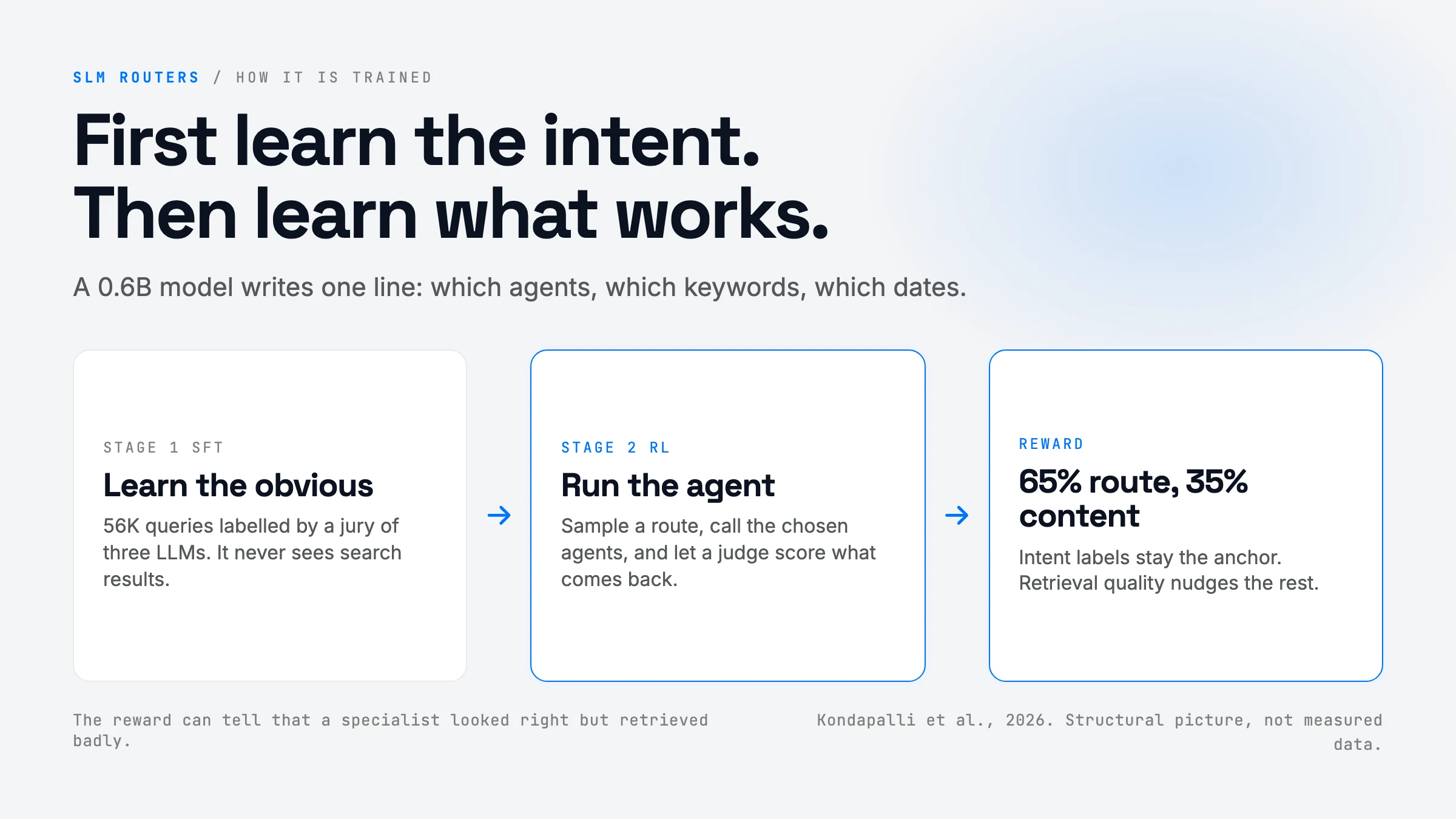
Stage 1: supervised fine-tuning (learn the obvious)
56K queries from production search logs plus synthetic ones, labelled by a jury of three LLMs (GPT-5, Claude Sonnet 4.6, Gemini 2.5 Pro). 80% were settled by majority vote; the rest were resolved by Sonnet, which a 100-query human check found best on dates and intent. Train Qwen3-0.6B with LoRA (rank 16, alpha 32, all attention + MLP projections), 2 epochs, LR 2e-4. Result: 89.4% exact source match, 96.7% keyword match, ~75 to 78% exact date match. This model is a good intent router. It still never sees retrieval results.
Stage 2: RL with a retrieval-grounded reward (learn what actually works)
For 11K fresh log queries: sample a routing line from the model (temperature 1.0 for diversity), actually run the chosen agent(s), score the outcome, update the policy with REINFORCE++, and keep it near the SFT model with a KL penalty of 0.15.
REINFORCE++ in one paragraph. Plain REINFORCE says: if an output got a better-than-usual reward, raise the probability of the tokens that produced it; if worse, lower it. “Better than usual” is the advantage: reward minus a baseline (here, normalised across the batch). REINFORCE++ adds PPO-style stabilisers (clipped updates, a per-token KL penalty, advantage normalisation) without training a separate value network, which is why it is cheap enough for a 0.6B model. The KL penalty is a leash: every step pays a cost for drifting from the SFT model, so RL refines routing without forgetting the format or the domain mapping.
The reward, demystified.
R = lambda_src x R_src + lambda_con x R_con, with lambda_src + lambda_con = 1 (the figure gives 0.65 / 0.35). Plain English: two thirds “did you route the way the intent labels say”, one third “did the agent you picked bring back good stuff”.
R_src = beta x P + gamma x D + (1 - beta - gamma) x K Plain English: routing quality blends three scores: P (did you pick the right agents), D (is the date window right) and K (are the keywords right). Each is in [0, 1].
P = clip(b + alpha_plus x |R+| - alpha_minus x |R-| + delta_miss, 0, 1) Plain English: start at a base score b. Add a bonus for each correct specialist you picked (R+), subtract a bigger penalty for each wrong specialist you picked (R-, since alpha_minus > alpha_plus), and if a specialist was needed and you picked none, subtract rho_m (delta_miss). Clamp to [0, 1]. What it does: it makes “spray every agent” a losing move, while still punishing “always fall back to web”.
D = f_date(q), K = f_keyword(q) Plain English: score the date window and keywords against the label. Both punish too narrow (misses results) and too broad (dilutes focus).
R_con = alpha x Rel + (1 - alpha) x Trust, with Rel = w_d r_direct + w_c r_complete + w_s r_semantic + w_f r_factual Plain English: an LLM judge reads what the agent returned and scores how directly it answers, how complete it is, how on-topic it is, how factually grounded it is, and how credible the sources are. What it does: this is the only term that sees the world. It is the term that can tell the model “genomics was on-topic but useless here”.
Why the mismatch detection emerges. For the PDB query, the SFT model and the labels may lean “genomics”. During RL the model samples both genomics and academic routes. Genomics earns a decent R_src but a near-zero R_con; academic earns a slightly lower R_src (if the label said genomics) but a high R_con. With enough samples of similar queries, academic’s total wins, its advantage is positive, and the policy shifts. The 0.65 weight on R_src means this only happens when the content gap is large, which is exactly the “clear mismatch” case.
Weights are not disclosed. Beyond the 0.65/0.35 split, every coefficient (b, alpha_plus, alpha_minus, rho_m, beta, gamma, alpha, the w’s) is called “tunable” with no values given. You will tune these yourself.
Architecture & data flow
flowchart LR
  Q[User query] --> R["Router SLM<br/>Qwen3-0.6B + LoRA"]
  R -->|"bitmask, keywords, dates"| P[Parse tool call]
  P --> A1[Academic agent]
  P --> A2[Finance agent]
  P --> A3["... 11 agents"]
  P --> A4[Web agent]
  A1 --> M[Merged ranked results]
  A2 --> M
  A3 --> M
  A4 --> M
  M --> U[Downstream LLM or user]
flowchart TD
  L["Search logs + synthetic queries"] --> J["LLM jury labels<br/>GPT-5, Sonnet 4.6, Gemini 2.5 Pro"]
  J --> SFT["Stage 1: SFT, 56K queries<br/>learn format + intent map"]
  SFT --> POL[Policy = SFT checkpoint]
  POL -->|"sample route, T=1.0"| RUN[Run selected agents]
  RUN --> JUDGE["LLM judge scores results<br/>R_con"]
  POL --> RS["Compare to labels<br/>R_src = P, D, K"]
  JUDGE --> REW["R = 0.65 R_src + 0.35 R_con"]
  RS --> REW
  REW --> UPD["REINFORCE++ update<br/>KL 0.15 to SFT"]
  UPD --> POL
Reward playground (schematic; coefficients are illustrative because the paper does not publish them). Pick a query, toggle which agents the router selects, and watch P, R_src, R_con and the total R change. On the PDB query, compare "genomics only" with "academic only": the intent term prefers genomics, but the content term flips the total.
The algorithm, simplified
# Stubs: router.sample(q) -> str line; run_agents(mask, kw, dates) -> list[doc]
#        judge(q, docs) -> dict of 0..1 scores; labels[q] -> gold mask/kw/dates
def reward(q, line, label, lam_src=0.65, b=0.5, a_plus=0.25, a_minus=0.4, rho=0.5):
    mask, kw, start, end = parse(line)            # "3 | Gene Therapy, Clinical Trials | 20240101 | 20241231"
    picked = {bit for bit in BITS if mask & bit}
    gold   = {bit for bit in BITS if label.mask & bit}
    right, wrong = (picked & gold) - {WEB}, (picked - gold) - {WEB}   # specialised routes only
    miss = -rho if (gold - {WEB}) and not (picked - {WEB}) else 0.0   # needed a specialist, picked none
    P = clip(b + a_plus * len(right) - a_minus * len(wrong) + miss, 0, 1)
    D = date_score(start, end, label)             # punish too-narrow and too-broad windows
    K = keyword_score(kw, label.keywords)         # embedding similarity
    R_src = 0.5 * P + 0.25 * D + 0.25 * K
    docs = run_agents(mask, kw, (start, end))     # THE new signal: actually retrieve
    s = judge(q, docs)
    rel = 0.4*s["direct"] + 0.2*s["complete"] + 0.2*s["semantic"] + 0.2*s["factual"]
    R_con = 0.8 * rel + 0.2 * s["trust"]
    return lam_src * R_src + (1 - lam_src) * R_con

def rl_step(router, sft_ref, batch, kl_coef=0.15):
    lines   = [router.sample(q, temperature=1.0) for q in batch]
    rewards = torch.tensor([reward(q, l, labels[q]) for q, l in zip(batch, lines)])
    adv     = (rewards - rewards.mean()) / (rewards.std() + 1e-6)   # better or worse than this batch
    logp    = router.logprob(batch, lines)        # [batch], summed over output tokens
    kl      = logp - sft_ref.logprob(batch, lines).detach()          # drift from SFT model
    loss    = -(adv * logp).mean() + kl_coef * kl.mean()
    loss.backward(); router.opt.step()
The weights inside reward are placeholders. The shape (intent-anchored, outcome-nudged, wrong specialists cost more than right ones earn) is the paper’s.
Built on Prior Work
| Prior idea | What it gave | What this paper changes |
|---|---|---|
| Federated search resource selection (Shokouhi & Si 2011) | Choosing which search engines to query from collection stats | Agents are tool-called with parameters; selection learned from per-query outcomes |
| ReSLLM (Wang et al. 2025) | LLMs as zero-shot resource selectors | Replaces the big LLM with a 0.6B model to get it off the latency budget |
| LTRR (Kim & Diaz 2025) | Rank retrievers by downstream utility | Domain-specialised agents with different data, plus joint parameter generation, trained by RL instead of feature LTR |
| Unsupervised RAG routing (Mu et al. 2025) | Use retrieved content to decide the best engine | Pays the “query everything” cost only at training time, not per request |
| DeepRetrieval (Jiang et al. 2025) | RL with retrieval metrics as reward, 3B model | Same reward idea, applied to which agent instead of how to rewrite the query |
| Cold-start SFT then RL (Wei et al. 2025) | SFT gives RL a sane starting policy | Applied to routing; KL leash to the SFT checkpoint |
| BEST-Route, Spotify query understanding (Palumbo et al.) | Multi-target routing; distil routing into small models | Bitmask multi-select; RL rather than pure distillation |
Results & Evidence
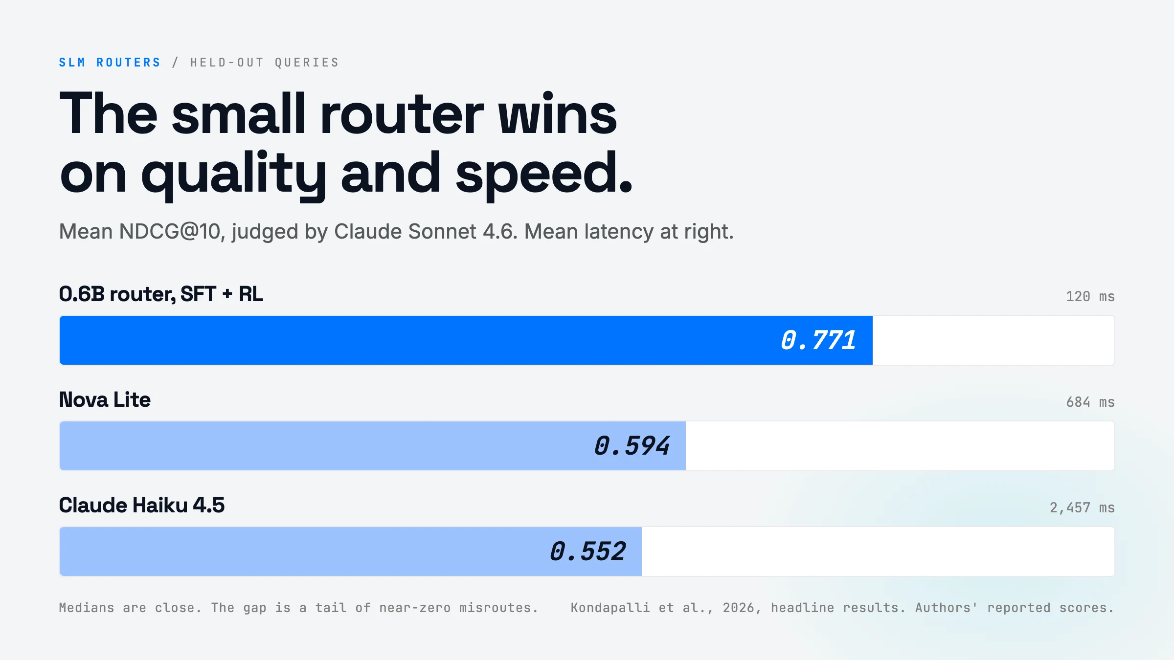
Headline numbers (held-out queries, Claude Sonnet 4.6 as blind relevance judge):
| SLM (SFT+RL) | Nova Lite | Haiku 4.5 | |
|---|---|---|---|
| Mean NDCG@10 | 0.771 | 0.594 | 0.552 |
| Median NDCG@10 | 0.960 | 0.926 | 0.929 |
| NDCG@10 on “redirect” subset | 0.918 | 0.539 | 0.490 |
| Mean latency | 120 ms | 684 ms | 2,457 ms |
| P99 latency | 179 ms | 4,659 ms | 6,985 ms |
SFT-only router: 89.4% source exact match, 115 ms. Base-model screening (no fine-tuning): Qwen3-0.6B got 30% fully-correct outputs; Llama 3.2 3B got 28% at 60 s per query.
How to read it. Medians are all ~0.93 to 0.96, so on easy queries every router is fine. The mean gap comes from a tail of queries scoring near 0 (whole result list judged irrelevant). The RL router has fewer of those. That is the real finding: fewer catastrophic misroutes, not better routing everywhere.
How NDCG@10 is computed in this paper. Click a result to cycle its judged grade (0 to 3). Note that the "ideal" ranking is built from the same 10 results, so a list of ten "marginal" results scores 1.0. NDCG here measures ordering and whether anything relevant came back, not how good the best possible answer was.
Caveats that matter:
- The redirect subset is selected by the winner. Table 4 is titled “queries where the router redirects away from specialised agents”. If the subset is defined by the SLM’s own behaviour, then of course the SLM looks best on it. Treat 0.918 vs 0.539 as an illustration, not a fair benchmark.
- One judge family everywhere. Sonnet 4.6 breaks label ties, an LLM judge supplies the RL content reward, and Sonnet 4.6 scores the evaluation. The router may be learning “what Sonnet likes” as much as “what is relevant”. No human relevance check on the final results.
- NDCG is normalised against the retrieved set itself (IDCG from the same 10 results). It cannot see a better document that the router’s choice failed to retrieve. A router that always gets “meh” results scores the same as one that gets great ones, as long as the order is right.
- No SFT-only NDCG. The paper says RL is what adds outcome awareness but only reports SFT on label-matching metrics. Without SFT-only NDCG we cannot separate “fine-tuning on in-domain logs” from “RL on retrieval reward”. This is the ablation you most want.
- Baselines are prompted LLMs only. No fine-tuned classifier, no LTRR, no RAGRoute, no “query all agents and rerank” upper bound. A LoRA-tuned 0.6B with the same 56K labels and no RL might already close most of the gap.
- Latency is not apples to apples. The SLM runs locally on an L4 via vLLM; Nova and Haiku are remote API calls, including network and queueing. The SLM still wins, but part of the 82% to 95% is deployment, not model.
- Small inconsistencies. Text says three base models were benchmarked, Table 1 lists four; SFT latency median (160.7 ms) is above its mean (133.9 ms) and P90; reward weights other than 0.65/0.35 are not given. One fixed pool of 11 agents, one company’s search logs.
What the evidence does establish: a 0.6B model can carry this whole routing-plus-parameters job inside a ~150 ms budget, and an outcome-aware reward plausibly reduces the “topically right, practically useless” misroute.
How You’d Use It
Your harness. If your agent loop has a “which tool / which sub-agent / which index” step that is a prompted call to a frontier model, that step is a candidate for this. Slot a small fine-tuned model in front of tool dispatch, outputting a compact structured line (mask + args), and keep the big model for reasoning. It improves latency per hop (seconds to ~100 ms) and makes routing deterministic enough to test. Cost: a GPU slot (an L4 class card is enough for 0.6B), a labelling pass, and an RL loop. It pays off when the router runs many times per task or many times per day, and when you have at least a few thousand real queries.
Your applications. Any product with multiple backends behind one search box (docs vs tickets vs code vs CRM; or legal vs finance vs news) has this exact problem. The concrete move: log for each query which source you hit and whether the user clicked, copied, or the downstream answer was accepted. That log is your R_con without an LLM judge. Even without RL, those logs let you find “topically right, practically wrong” sources and hand-fix them. What must be true: real traffic, and a usable outcome signal per query.
Your automations and business processes. Document intake pipelines (route an inbound file to the right extractor or queue) suffer the same failure: the “invoice” classifier sends a credit memo to the invoice extractor, which then fails. Use the downstream extractor’s success (fields validated, no human correction) as the reward and RL-tune the classifier toward routes that actually complete. It improves straight-through rate; it costs an outcome hook on each extractor.
Your workflows and methodologies. The transferable habit: score routers on what they cause, not on label agreement. When you evaluate any dispatcher (model router, tool picker, sub-agent selector), measure end-task quality per route and look at the bottom 10% of queries, not the median. This paper’s mean-vs-median split shows the median hides everything.
Build Your Own (Minimal Recipe)
Components
- Output schema. A one-line format:
mask | kw1, kw2 | start | end. Keep it tiny; parse it strictly; reject malformed lines. - Labels. 5K to 50K real queries. Label with 2 to 3 LLMs by majority vote; resolve disagreements with your best judge; hand-check 100.
- SFT. Qwen3-0.6B (or 1.7B if you can afford ~2x latency) with Unsloth + LoRA r=16. 2 epochs. Check exact-match on a held-out split. Stop here first and measure end-task quality: this alone may be enough.
- Outcome reward. For each sampled route, run the agents (cache aggressively: same query + same mask gives the same results), then score with a judge or, better, with real outcome signals.
- RL. OpenRLHF or TRL with REINFORCE++ / GRPO, KL ~0.1 to 0.2 to the SFT checkpoint, temperature 1.0, small LR (5e-6).
- Serve. vLLM, short max tokens, constrained decoding to the schema.
Build order: schema, then labels, then SFT, then an end-to-end eval harness (NDCG or task success per route, with a separate judge from training), then RL, then compare SFT vs SFT+RL on that harness.
The hard parts
- Reward cost and noise. Every RL sample means real retrieval plus a judge call. Precompute: for each training query, run all agents once and judge each result set. Then RL reads rewards from a table, which is fast and lets you sample freely. With 11 agents and single-agent routes this is 11 calls per query; multi-agent masks can be scored by merging cached single-agent results.
- Not training on the judge’s taste. Use a different judge for evaluation than for reward, and spot-check with humans or real user outcomes.
Libraries/models: Qwen3-0.6B/1.7B, Unsloth (SFT), OpenRLHF or TRL (RL), vLLM (serving), Outlines or vLLM guided decoding (schema), gte-base (keyword similarity), any strong LLM as judge.
How to Improve It
- Run the missing ablation. SFT-only vs SFT+RL vs RL-only on the same NDCG harness, with a different judge and a redirect subset defined before looking at router outputs. If SFT-only gets most of the gain, you can skip RL entirely.
- Skip the label anchor where you have outcomes. Precompute per-agent quality for each training query and train directly on “best agent by measured quality” (a contextual bandit or listwise target). That removes the dependence on intent labels that may be wrong in the very cases you care about.
- Condition on agent descriptions. Put a short capability card per agent in the prompt (the authors’ own suggested next step) so new agents can be added without retraining, and train with random agent subsets so the model learns to read cards rather than memorise bit positions.
- Add an “ask for more” action. Let the router output a confidence or a “try two agents” fallback when uncertain, and reward the cost-quality trade-off explicitly (penalty per extra agent call). That turns the static alpha_minus penalty into a learned budget.
- Use real outcome signals instead of an LLM judge. Clicks, dwell, accepted answers, or downstream task success are cheaper and harder to game. Mix them with the judge and watch for disagreement.
Glossary
- SLM — small language model; here 0.6B parameters, small enough for ~100 ms on one modest GPU.
- Router / agent selection — the step that decides which specialised retrieval agent(s) a query goes to.
- SFT — supervised fine-tuning: train on input-output pairs so the model copies the labelled answers.
- RL (reinforcement learning) — train by sampling outputs, scoring them with a reward, and making high-scoring outputs more likely.
- REINFORCE++ — a simple policy-gradient RL method with PPO-style stabilisers and no separate value model.
- Advantage — how much better an output’s reward is than the batch average; positive means “do more of this”.
- KL penalty — a cost for drifting away from a reference model’s probabilities; keeps RL from breaking what SFT taught.
- LoRA — fine-tuning a small set of added low-rank weights instead of the whole model; cheap and fast.
- Bitmask — encoding a set of choices as one integer where each agent is one bit (web=1, academic=2, …).
- NDCG@10 — a 0 to 1 ranking score over the top 10 results that rewards putting highly relevant items first.
- IDCG — the best possible DCG for a given set of results; NDCG divides by it.
- LLM-as-judge — using an LLM to grade relevance or quality instead of human annotators.
- Intent-based routing — choosing an agent from what the query is about, without seeing results.
- Federated search / resource selection — the classic IR problem of picking which search engines to query.
- P99 latency — the time under which 99% of requests finish; the worst-case users actually feel.
- vLLM — a fast open-source inference server for LLMs.